Using the Iris and SOL programs, sunspots positions can be measured almost automatically. During this process, it is hardly necessary to know how Iris works, given that SOL acts as an intermediary between the program and us.
Here the process is described as it would be done exclusively by Iris (the names of the menus will be indicated in English, followed by parentheses, of the name of the French version).
Conversion of the images
The processing is done from a sequence of images in RAW format, which must be converted to FIT as explained in http://www.parhelio.com/en/docposic.html. Only add that Iris takes the first image (a1) of the series, as a reference to align the others, but that image will be on the edge of the field, where there is more vignetting. In addition, the last image will be at the other end, and Iris may encounter difficulties if the distances are large. For these reasons, it is a good idea to exchange one of the central images for the first one. For example, if there are 40 images, we call "a1" "a20", and "a20" we call it "a1".
Alignment of images
Iris has a very effective tool to align disks so, in the case that concerns us, we use the command >cregister. In each image, this command adjusts a circle to the pixels that have a certain intensity, calculates the coordinates of the center of that circle, and then moves the image so that the center coincides with that of the first image.
What intensity do we use for the adjustment? SOL calculates the intensity of the limbus from the histogram. However, if we do it manually, it is best to open the first image by typing in the command window:
>load a1
Then, in the "View" menu ("Visualization") we mark "Slice" ("Coupe"). This option is used to measure the intensities along a line. Holding down the left mouse button, we draw a line that crosses the entire disk, and when you release it, a graph with these intensities will appear:
Alineamiento de las imágenes
Iris dispone de una herramienta muy eficaz para alinear discos por lo que, en el caso que nos ocupa, utilizamos el comando >cregister. En cada imagen, dicho comando ajusta un círculo a los píxeles que tengan una determinada intensidad, calcula las coordenadas del centro de ese círculo, y luego desplaza la imagen para que dicho centro coincida con el de la primera imagen.
¿Qué intensidad utilizamos para el ajuste? Sol calcula la intensidad del limbo a partir del histograma. Sin embargo, si lo hacemos manualmente lo mejor es abrir la primera imagen, escribiendo en la ventana de comandos:
>load a1
A continuación, en el menú "View" ("Visualisation") marcamos "Slice" ("Coupe"). Esta opción sirve para medir las intensidades a lo largo de una línea. Manteniendo pulsado el botón izquierdo del ratón, trazamos una línea que cruce todo el disco, y al soltarlo, aparecerá una gráfica con dichas intensidades:
We can see how the intensity decreases towards the limbus, and the fact that the darkening is not symmetrical is due to light clouds and some vignetting. If we take a very high intensity, those factors can influence the adjustment and subsequent alignment. In this example, a value of 200-250 can serve us perfectly. If we now execute >cregister we will see how the program is aligning the images:
>cregister a b 200 39
where "a" is the generic name of the initial series, "b" the name of the series already aligned; "200", the intensity of adjustment, and "39" the number of images. To add them:
>add_norm b 39
As the resulting image will appear saturated, in the "Threshold" box ("Seuils de visualisation") we will move the upper cursor to the extreme right, and save the image:
>save c
Orientation of the image
The most important thing of the previous process, is that the file Shift.lst has been created in the working folder of Iris, which contains the displacements suffered by each image to make them coincide. Now, if we consider as the origin of coordinates, the center of the disk of the first image; then these displacements are the coordinates of the centers of all the disks, changed sign. This information is crucial, because if we adjust that cloud of points by least squares, the slope gives us the orientation of the image, and therefore, what angle we have to turn it so that the north celestial is above.
When we represent the data of Shift.lst, we obtain a graph as the inferior one; and if we use Excel, we can use the "Pending" function. Another option is to add a "trend line", choosing the linear type, and showing the equation in the graph. The result for our example is shown below:
The slope in this case is m = 0.0595, and therefore, the angle would be A = arctg 0.0595 = 3º4
Now we need two things: the angles P, B0 and L0, which we will find in some ephemeris, and the coordinates of the center of the disk and its radius. To do this, we repeat the previous operation drawing a line that crosses the disk and choosing an appropriate intensity. Since we now have a sum instead of an individual image, the intensities in the whole image will be higher. In the "View" menu ("Visualization"), we can uncheck "Slice" ("Coupe") and insert the entire disk by holding down the left mouse button. Then we execute the command >circle:
>circle 4000
where 4000 is the intensity chosen. In the output window we will see the coordinates of the center and the radius appear (all in pixels):
If we have difficulty selecting the whole disk because it overflows the screen, we can use the command >mouse_select. For example:
> mouse_select 1 1 xmax ymax
where "xmax" and "ymax" are the dimensions of the image in pixels or a slightly lower figure.
SOL determines the center and radius of the disc with two slightly different intensities, which gives an idea of the clarity with which the limb appears. If the radii corresponding to both intensities are very different, the image is probably out of focus or misaligned, and will not be suitable for measuring positions.
Now, with the >rot command, we first correct the angle A and then the angle P:
>rot X Y -A
>rot X Y -P
where (X, Y) are the coordinates of the center of the disk. The angles are changed sign because it is a correction, that is, you have to cancel the effect that both have on the inclination of the image.
In all this analysis we are assuming that, as seen by the camera viewer, the North is up and the East is on the left, that is, the Sun moves from left to right along the image. However, we could be using an optical configuration that produces some inversion and in that case, we must correct it.
If the North is in the lower zone, we must do:
>rot X Y A
>rot X Y P
>mirrorx
If the East is on the right:
>rot X Y A
>rot X Y P
>mirrory
If the North is below and the East to the right, then:
>rot X Y -A
>rot X Y -P
>mirrorx
>mirrory
Once oriented, it is convenient to get the center and the radius on this last image, because there are usually small variations.
Creation of a template
Iris is prepared to obtain ephemeris of Mars and Jupiter and, from them, can create a template. However, it can not do it with the Sun and, in addition, unlike with Mars and Jupiter, in the Sun the length increases towards the West. However, with certain premises, we can adapt a template created by the program and use it with the Sun. Let's see how.
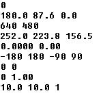 |
The program saves the parameters of the template in a text file with extension lst. The content occupies 10 lines, of which, the last one must be left blank (this detail is important because otherwise the program will not recognize the file). The easiest thing is to copy the contents of the image on the left in Notepad and, once saved, change the extension to lst. Of all the numbers, the ones that interest us most are those that appear in the 2nd, 3rd, 4th and last line:
2nd line: the first number is 0 if the latitude of the center of the disk (B0) is positive and 180 if B0 is negative. The 2nd number is 90-B0. The 3rd number is the length of the central meridian (L0). To avoid the problem of the length mentioned above, it is preferable that it is always 0. In this way, the program will give us the differences in length between the spot and the meridian.
3rd line: Size of the photo (in pixels).
4th line: The first two numbers are the coordinates (X, Y) of the center of the disk and the third is the radius.
Last line: The first 2 values are the difference in degrees between two meridians or consecutive parallels of the template. The last one we left as 1.
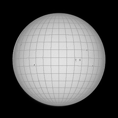
Once this file is saved in the Iris work folder, we execute the following command:
> grid sun 5000
where "sun" is the name of the lst file and 5000 the intensity of the template. The result we see in the following image:
 |
Medida de posiciones
Con la plantilla ya podemos obtener posiciones aproximadas. Sin embargo, con Iris podemos conseguir coordenadas mucho más precisas determinando los centros fotométricos de las manchas. Para ello, rodeamos una mancha con un pequeño rectángulo, pinchamos en la imagen con el botón derecho y después en "Statistics" ("Statistiques").
Measurement of positions
With the template we can already obtain approximate positions. However, with Iris we can achieve much more precise coordinates by determining the photometric centers of the spots. To do this, we surround a spot with a small rectangle, click on the image with the right button and then "Statistics" ("Statistiques").
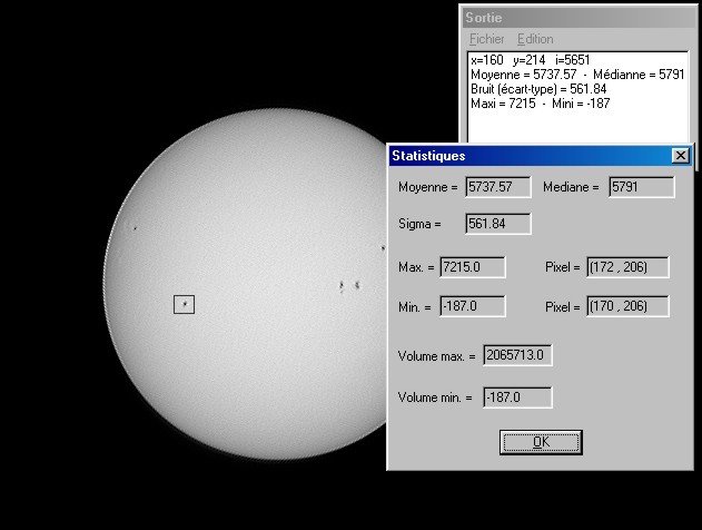 |
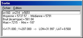
The box that comes out gives us the position of the pixel of minimum intensity within the rectangle (170, 206). Now we execute:
>rec2map sun 170 206
and the program returns the position of the spot in the output window. Recall that the length is, in reality, the difference with the central meridian. Knowing L0, the calculation of the heliographic length is immediate.